The KdV Equation and Solitons

The KdV Equation and Solitons

Here $u(x,t):\mathbb R\times[0,\infty)\to\mathbb R$ represents the evolution of the height of a $1D$ fluid (in a moving frame, so don't expect $x\mapsto -x$ symmetry)

Here $u(x,t):\mathbb R\times[0,\infty)\to\mathbb R$ represents the evolution of the height of a $1D$ fluid (in a moving frame, so don't expect $x\mapsto -x$ symmetry)

Here $u_t,u_x, u_{xxx},\ldots$ denote the partial derivatives $\partial_tu,\partial_xu,\partial_{x}u,\partial_{xxx} u\ldots$

Here $u_t,u_x, u_{xxx},\ldots$ denote the partial derivatives $\partial_tu,\partial_xu,\partial_{x}u,\partial_{xxx} u\ldots$

The Linear Case and the Superposition Problem

The Linear Case and the Superposition Problem

Look at e.g. a linear PDE of the form $u_t=Lu$ or $u_{tt} = L u$, where $L$ is linear operator, i.e. a linear function of $u,u_{x},u_{xx},u_{xxx}, \ldots$

Look at e.g. a linear PDE of the form $u_t=Lu$ or $u_{tt} = L u$, where $L$ is linear operator, i.e. a linear function of $u,u_{x},u_{xx},u_{xxx}, \ldots$

In particular, if we can diagonalize $L$, we can find some 'basic' solutions associated with the eigenbasis of $L$

In particular, if we can diagonalize $L$, we can find some 'basic' solutions associated with the eigenbasis of $L$

Then we can write the initial conditions as a (generalized) linear combination of eigenfunctions, and we evolve them (note that if we have a second-order in time, we need a velocity initial condition as well)

Then we can write the initial conditions as a (generalized) linear combination of eigenfunctions, and we evolve them (note that if we have a second-order in time, we need a velocity initial condition as well)

The KdV equation reads

The KdV equation reads

$u_t - 6 u u_x + u_{xxx} = 0$

So, by the above we mean:

So, by the above we mean:

With initial condition $u_0$

With initial condition $u_0$

$\partial_t u(x, t)=6u(x, t) \partial_x u(x) + \partial_{xxx} u(x, t)$

$u(x,0)=u(x)\,\,\forall x\in \mathbb R$

If we have solutions then any linear combination of these solutions is also one (that's sometimes called the superposition principle)

If we have solutions then any linear combination of these solutions is also one (that's sometimes called the superposition principle)

This will be useful later, but for now it helps us appreciate the behavior of (some particular solutions) to KdV equation, which is _nonlinear_

This will be useful later, but for now it helps us appreciate the behavior of (some particular solutions) to KdV equation, which is nonlinear

Scattering and Inverse Scattering Transforms

Scattering and Inverse Scattering Transforms

$u(\cdot,t)=\mathcal{IST}[\mathrm{Evol}_{0\leadsto t}[\mathcal{ST}[u(\cdot,0)]]]$

Goals of the scattering transform

Goals of the scattering transform

The claim is that there scattering transform $\mathcal{ST}$ acting on functions and an inverse scattering transform $\mathcal {IST}$ such that the scattering data (the result of the scattering transform) evolves very nicely in time

The claim is that there scattering transform $\mathcal{ST}$ acting on functions and an inverse scattering transform $\mathcal {IST}$ such that the scattering data (the result of the scattering transform) evolves very nicely in time

where the evolution $\mathrm{Evol}_{0\leadsto t}$ of the scattering data is very simple

where the evolution $\mathrm{Evol}_{0\leadsto t}$ of the scattering data is very simple

For the heat equation $h_t(x,t)=h_{xx}(x,t)$, where if compute the Fourier transform $\mathcal F$ (with respect to space), since $\mathcal F(h_{xx})(\xi)=-\xi^2 \mathcal F(h)(\xi)$ (integrate by parts twice), we solve the ODE for fixed $\xi$ with respect to $t$ and find a very simple evolution for the Fourier transform:

For the heat equation $h_t(x,t)=h_{xx}(x,t)$, where if compute the Fourier transform $\mathcal F$ (with respect to space), since $\mathcal F(h_{xx})(\xi)=-\xi^2 \mathcal F(h)(\xi)$ (integrate by parts twice), we solve the ODE for fixed $\xi$ with respect to $t$ and find a very simple evolution for the Fourier transform:

So, to compute the solution of the heat equation at time $t$, we just take the inverse Fourier transform of $F(h(\cdot,t))$, and that's it

So, to compute the solution of the heat equation at time $t$, we just take the inverse Fourier transform of $F(h(\cdot,t))$, and that's it

$\mathcal F(h(\cdot,t))=e^{-\xi^2 t}\mathcal F(h(\cdot,0))$

Obviously, this is because we have a linear equation: we basically found a 'basis' of solutions $x\mapsto e^{i\xi x}$ that evolve nicely in time and because the equation is linear, if we can represent things as sum of them at time $t=0$ (as the Fourier transform does), then the evolution is simply the sum of the evolution of the 'components' $e^{i\xi x}$

Obviously, this is because we have a linear equation: we basically found a 'basis' of solutions $x\mapsto e^{i\xi x}$ that evolve nicely in time and because the equation is linear, if we can represent things as sum of them at time $t=0$ (as the Fourier transform does), then the evolution is simply the sum of the evolution of the 'components' $e^{i\xi x}$

In other words, we broke the solution into independent pieces, each of which evolves independently

In other words, we broke the solution into independent pieces, each of which evolves independently

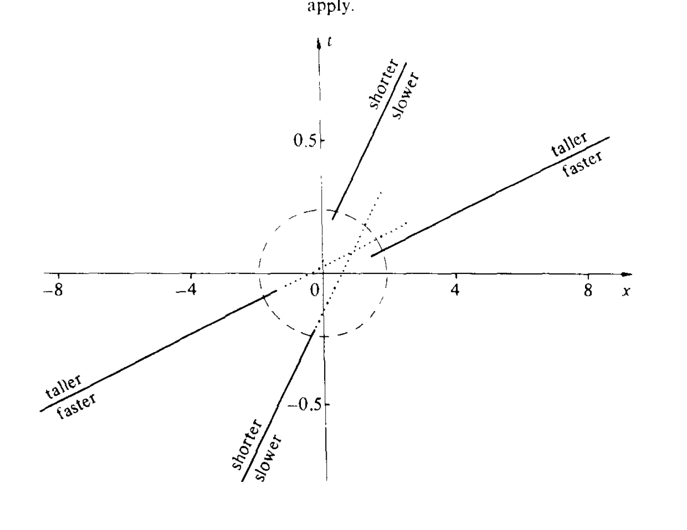
But of course, none of this can work if the equation is nonlinear... and that's what make things interesting (and it's not because it's harder): if we take the sum of two KdV waves, the result of their evolution won't be the sum of their evolution: the point is that they interact

But of course, none of this can work if the equation is nonlinear... and that's what make things interesting (and it's not because it's harder): if we take the sum of two KdV waves, the result of their evolution won't be the sum of their evolution: the point is that they interact

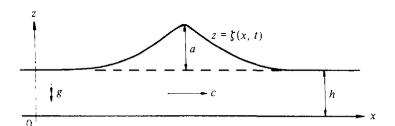
If we take as initial condition $u(x,0)=-\frac c 2 \mathrm{sech}^2(\frac {\sqrt c}{2}(x-x_0))$, for some $c>0$ and some $x_0\in\mathbb R$ with $\mathrm {sech} = 1/\cosh$, then the solution for all $t\geq 0$ is $u(x,t)=-\frac c 2\mathrm{sech}^2(\frac{\sqrt c}{2}(x-ct-x_0))$

If we take as initial condition $u(x,0)=-\frac c 2 \mathrm{sech}^2(\frac {\sqrt c}{2}(x-x_0))$, for some $c>0$ and some $x_0\in\mathbb R$ with $\mathrm {sech} = 1/\cosh$, then the solution for all $t\geq 0$ is $u(x,t)=-\frac c 2\mathrm{sech}^2(\frac{\sqrt c}{2}(x-ct-x_0))$

A particular solution with one soliton

A particular solution with one soliton

A particular solution with two solitons

A particular solution with two solitons

How the heat equation was solved by Fourier

How the heat equation was solved by Fourier

The Delay Phenomenon

The Delay Phenomenon

How can we have the idea that KdV is solvable?

How can we have the idea that KdV is solvable?

It is not the most obvious idea in the world, but it is generally acknowledged that once we understand that the KdV equation has a so-called Lax pair formulation, then this makes us optimistic

It is not the most obvious idea in the world, but it is generally acknowledged that once we understand that the KdV equation has a so-called Lax pair formulation, then this makes us optimistic

What is the Lax Pair formulation?

What is the Lax Pair formulation?

Key Points to Explain

Key Points to Explain

What is the scattering transform? What does it transform $u:\mathbb R\to \mathbb R$ into?

•

What is the scattering transform? What does it transform $u:\mathbb R\to \mathbb R$ into?

How do we see the solitons emerge in the scattering transform?

•

How do we see the solitons emerge in the scattering transform?

Why is there a finite number of solitons in the scattering transform?

•

Why is there a finite number of solitons in the scattering transform?

Why is the scattering transform invertible?

•

Why is the scattering transform invertible?

Why is the scattering data evolving so simply through the KdV equation?

•

Why is the scattering data evolving so simply through the KdV equation?

How do we identify solitons and bound states associated with the scattering transform?

•

How do we identify solitons and bound states associated with the scattering transform?

Given the scattering data, how can we reconstruct $u$?

•

Given the scattering data, how can we reconstruct $u$?

What is the Scattering Transform, physically?

What is the Scattering Transform, physically?

For a given $u:\mathbb R\to\mathbb R$ that decays at infinity, we are going to consider the physical process of [1] thinking of $u$ as a potential of a material [2] sending waves from $-\infty $ to $+\infty$ through a material with potential $u$

For a given $u:\mathbb R\to\mathbb R$ that decays at infinity, we are going to consider the physical process of [1] thinking of $u$ as a potential of a material [2] sending waves from $-\infty$ to $+\infty$ through a material with potential $u$

What we do intuitively is: extract the data of how waves of various frequencies get transmitted and reflected going through the material with potential $u$; we call these _transmission and reflection coefficients_

▸

What we do intuitively is: extract the data of how waves of various frequencies get transmitted and reflected going through the material with potential $u$; we call these transmission and reflection coefficients

To be more complete, we also send signals that grow exponentially through the material and see if they die out (this happens for only a finite number of growth rate); we call these _bound states_

▸

To be more complete, we also send signals that grow exponentially through the material and see if they die out (this happens for only a finite number of growth rate); we call these bound states

The _scattering data_ is the data of the transmission and reflection coefficients and of the bound states

•

The scattering data is the data of the transmission and reflection coefficients and of the bound states

The operation to describe a potential $u$ by its scattering data is injective: from the scattering data, we can fully reconstruct $u$ (something that may or may not be intuitive, but is really not obvious!)

The operation to describe a potential $u$ by its scattering data is injective: from the scattering data, we can fully reconstruct $u$ (something that may or may not be intuitive, but is really not obvious!)

There is the Lax Pair formulation:

There is the Lax Pair formulation:

$ \partial_t L_u=[A,L_u] $

$A_v=-4\partial_{xxx}+6v\partial _x+3v_x$

$L_v=-\partial_{xx}+v$

The operation $[X,Y]=XY-YX$ is the infinitesimal version of the conjugation:

The operation $[X,Y]=XY-YX$ is the infinitesimal version of the conjugation:

So the equation $\partial t X = [Y,X]$ says that $X$ undergoes a progressive change of basis

So the equation $\partial t X = [Y,X]$ says that $X$ undergoes a progressive change of basis

The eigenvectors move like $\partial_t \psi=A\psi$

The eigenvectors move like $\partial_t \psi=A\psi$

If we define the two operations $A_u$ and $L_u$ that are functions of a function $v:\mathbb R \to \mathbb R$ and that act on functions $\mathbb R \to \mathbb R$

If we define the two operations $A_u$ and $L_u$ that are functions of a function $v:\mathbb R \to \mathbb R$ and that act on functions $\mathbb R \to \mathbb R$

Then if we make things evolve in time and take $v(x)$ to be equal to $u(x,t)$ we have that the Lax equation $\partial_t A_u=[L_u,A_u]=L_u A_u -A_u L_u$ corresponds to the KdV equation (easy computation)

Then if we make things evolve in time and take $v(x)$ to be equal to $u(x,t)$ we have that the Lax equation $\partial_t A_u=[L_u,A_u]=L_u A_u -A_u L_u$ corresponds to the KdV equation (easy computation)

In other words, if we want that the Lax equation $\partial_t A_u=[L_u,A_u]$ holds true, then $u$ must _evolve_ in time like the $u$ solving the KdV equation

In other words, if we want that the Lax equation $\partial_t A_u=[L_u,A_u]$ holds true, then $u$ must evolve in time like the $u$ solving the KdV equation

What does the Lax equation mean?

What does the Lax equation mean?

So, the spectrum doesn't change, and the eigenfunctions change progressively

So, the spectrum doesn't change, and the eigenfunctions change progressively

What should we do, then?

What should we do, then?

We should study the spectrum and eigenfunctions of the so-called _Schrödinger operator_

We should study the spectrum and eigenfunctions of the so-called Schrödinger operator

$(\mathrm{Id}+\epsilon X)Y(\mathrm{Id}+\epsilon X)^{-1}=Y+\epsilon[X,Y]+O(\epsilon^2)$

$L_u=-\partial_{xx} +u$

So that this is clear:

So that this is clear:

$A_v\psi(x)=-4\partial_{xxx} \psi(x)+6v(x)\psi'(x)+3 v_x(x)\psi(x)$

$L_v\psi(x)=-4\psi''(x)+v(x)\psi(x)$

Since if $u$ follows the KdV equation, the spectrum of $L_u$ (whatever this means) is not expected to change, and the eigenfunctions should change nicely

Since if $u$ follows the KdV equation, the spectrum of $L_u$ (whatever this means) is not expected to change, and the eigenfunctions should change nicely

What can we say about the spectrum a priori?

What can we say about the spectrum a priori?

If we look at what happens with $u\equiv0$ then there are no $L^2$ eigenfunctions (of finite norm):

If we look at what happens with $u\equiv0$ then there are no $L^2$ eigenfunctions (of finite norm):

The operator is 'formally self-adjoint', i.e. $\lang L_u \psi,\phi\rang=\bar{\lang\psi,L_u \phi\rang}$, for $\lang \phi,\psi\rang=\int_{-\infty}^{+\infty} \bar \phi (x)\psi(x) dx$

The operator is 'formally self-adjoint', i.e. $\lang L_u \psi,\phi\rang=\bar{\lang\psi,L_u \phi\rang}$, for $\lang \phi,\psi\rang=\int_{-\infty}^{+\infty} \bar \phi (x)\psi(x) dx$

So, the eigenfunctions are likely to be real

So, the eigenfunctions are likely to be real

If we look for negative eigenvalues and try to solve $-\partial_{xx}\psi(x)=-k^2\psi(x)$ (the eigenvalue $\lambda=k^2$), we find $\psi(x)=e^{ikx}$ and $\psi(x)=e^{-kx}$, which are nice, but definitely not in $L^2$ (not finite norm)

If we look for negative eigenvalues and try to solve $-\partial_{xx}\psi(x)=-k^2\psi(x)$ (the eigenvalue $\lambda=k^2$), we find $\psi(x)=e^{ikx}$ and $\psi(x)=e^{-kx}$, which are nice, but definitely not in $L^2$ (not finite norm)

If we look for positive eigenvalues, we should have something like $\psi(x)=e^{kx}$, and this has no chance of being of finite norm

If we look for positive eigenvalues, we should have something like $\psi(x)=e^{kx}$, and this has no chance of being of finite norm

Solving an ODE to find eigenfunctions

Solving an ODE to find eigenfunctions

No matter what $u$ is, it is clear the for fixed $\lambda\in\mathbb C$, we can try to solve $L_u \psi=\lambda \psi$, because this amounts to solving a second-order ODE

No matter what $u$ is, it is clear the for fixed $\lambda\in\mathbb C$, we can try to solve $L_u \psi=\lambda \psi$, because this amounts to solving a second-order ODE

$\psi''(x)=(u(x) - \lambda)\psi(x)$

And this always has a two-dimensional space of solutions

And this always has a two-dimensional space of solutions

If $|u(x)|\to 0$ as $|x|\to\infty$, then at infinity we have the solutions $e^{ikx}$ and $e^{-ikx}$

If $|u(x)|\to 0$ as $|x|\to\infty$, then at infinity we have the solutions $e^{ikx}$ and $e^{-ikx}$

Also, if we try to find a real, bounded solution, we can try to find something of the form $e^{kx}$ at $x\to-\infty$ (decaying at $-\infty$) and of the form $e^{-kx}$ at $x\to +\infty$ (decaying at $+\infty)$, and hope that they can be 'pasted': generically this will not happen (there would be a discontinuity of the solution or its derivative), but for some exceptional cases, this will work

Also, if we try to find a real, bounded solution, we can try to find something of the form $e^{kx}$ at $x\to-\infty$ (decaying at $-\infty$) and of the form $e^{-kx}$ at $x\to +\infty$ (decaying at $+\infty)$, and hope that they can be 'pasted': generically this will not happen (there would be a discontinuity of the solution or its derivative), but for some exceptional cases, this will work

In fact, these exceptional cases correspond to so-called _bound states_ of the operator $L_u$, and they correspond to positive eigenvalues, there is a finite number of them, in fact they correspond to each of the solitons in $u$

In fact, these exceptional cases correspond to so-called bound states of the operator $L_u$, and they correspond to positive eigenvalues, there is a finite number of them, in fact they correspond to each of the solitons in $u$

(If we believe this, then this explains why the number of solitons is preserved: the spectrum of $L_u$ stays constant as $u$ evolves through KdV)

(If we believe this, then this explains why the number of solitons is preserved: the spectrum of $L_u$ stays constant as $u$ evolves through KdV)

The eigenvectors move like $\partial_t \psi=Y\psi$, in fact

The eigenvectors move like $\partial_t \psi=Y\psi$, in fact

(By the Lax equation, $\partial_t \psi=A_u\psi$)

(By the Lax equation, $\partial_t \psi=A_u\psi$)

So, what do we do?

So, what do we do?

We study the structure of the eigenfunctions of $L_u$, and we realize this amounts to in fact understanding the wave equation in medium $u$ for some auxiliary time $\tau\in\mathbb R$ (which has nothing to do with the time of KdV

We study the structure of the eigenfunctions of $L_u$, and we realize this amounts to in fact understanding the wave equation in medium $u$ for some auxiliary time $\tau\in\mathbb R$ (which has nothing to do with the time of KdV

$\partial_{\tau\tau} \psi(x,\tau)+L_u\psi(x,\tau)=0$

Why? Because what if we tried to solve this wave equation in medium $u$, we would be exactly trying to diagonalize $L_u$

Why? Because what if we tried to solve this wave equation in medium $u$, we would be exactly trying to diagonalize $L_u$

If we write things explicitly, so that we are not confused:

If we write things explicitly, so that we are not confused:

$\partial_{\tau\tau} \psi(x,\tau, t) = -u(x,t) \psi(x,\tau, t) + \partial_{xx} \psi(x,\tau, t)$

Now: the Scattering Transform!

Now: the Scattering Transform!

The physical idea is to send waves of various frequencies from $-\infty$, see how much they get reflected back to $-\infty$ and transmitted to $+\infty$

The physical idea is to send waves of various frequencies from $-\infty$, see how much they get reflected back to $-\infty$ and transmitted to $+\infty$

This will define some _reflection_ and $transmission$ coefficients, and we will relate them to the 'spectral data' of $L_u$ (basically from them, we can construct eigenfunctions, so they are the spectral data, really)

This will define some reflection and $transmission$ coefficients, and we will relate them to the 'spectral data' of $L_u$ (basically from them, we can construct eigenfunctions, so they are the spectral data, really)

We will also have a few _bound_ states, i.e. things that we make grow exponentially from $-\infty$ and that don't explode after traversing the medium: they decay exponentially going to $+\infty$

We will also have a few bound states, i.e. things that we make grow exponentially from $-\infty$ and that don't explode after traversing the medium: they decay exponentially going to $+\infty$

Now, the good news is that the spectral data (the reflection & transmission coefficients, and the spectral data) evolve nicely

Now, the good news is that the spectral data (the reflection & transmission coefficients, and the spectral data) evolve nicely

And from there, to truly solve the KdV equation we will have the task to _recover the medium_ from the scattering data and bound states: this is the _inverse scattering transform_

And from there, to truly solve the KdV equation we will have the task to recover the medium from the scattering data and bound states: this is the inverse scattering transform

Note that the problem is of independent interest: it's interesting to know that we can know a medium from the way it reflects and transmits frequencies

Note that the problem is of independent interest: it's interesting to know that we can know a medium from the way it reflects and transmits frequencies

Finally, at some point, we need to explain how the solitons can be understood from the bound state data

Finally, at some point, we need to explain how the solitons can be understood from the bound state data

(Summary of the above)

(Summary of the above)

Scattering Data Evolution in KdV time $t$

Scattering Data Evolution in KdV time $t$

$d_t R^{(k)}-4ik^3R^{(k)}=4ik^3R^{(k)}$

$d_tT^{(k)}+4ik^3T^{(k)}=4ik^3T^{(k)}

d_tT^{(k)}+4ik^3T^{(k)}=4ik^3T^{(k)}

$R^{(k)}(t)=R^{(k)}(0)\exp(8ik^3t)$

$T^{(k)}(t)=T^{(k)}(0)$

$\partial_t\log\psi^{(n)}=-u_x-2(u-2\kappa_n^2)\partial_x\log\psi^{(n)}$

$R^{(n)}=\psi^{(n)}_t+u_x\psi^{(n)}-2(u-2\kappa_n^2)\psi_x^{(n)}=0$

$d_t c_n(t)-4\kappa_n^3c_n(t)=0$

$c_n(t)=c_n(0)\exp(4\kappa_n^3t)$

Bound State Data

Bound State Data

Reflection and Transmission Coefficient Data

Reflection and Transmission Coefficient Data

$u=-2d_xK(x,x)$

$u:\mathbb R\to\mathbb R$

$\phi_{\tau \tau}+L_u\phi=0$

$L_u=(-\partial_{xx}+u)$

Think we are sending waves through a medium with potential $u$ and observing what happens to study $u$

Think we are sending waves through a medium with potential $u$ and observing what happens to study $u$

$\{(\psi,\lambda):L_u\psi=\lambda \psi\}$

$K(x,\tau)$: $K(x,\tau)=0$ if $x>\tau$

$K(x,\tau)$: $K(x,\tau)=0$ if $x>\tau$

If we send a Dirac wave from $-\infty$ at time $-\infty$ through a medium with potential $u$, so that the wave front travels at unit speed rightwards, $K(x,\tau)$ is the amount of 'stuff' scattered behind the wave front at position $x$ at time $\tau$

If we send a Dirac wave from $-\infty$ at time $-\infty$ through a medium with potential $u$, so that the wave front travels at unit speed rightwards, $K(x,\tau)$ is the amount of 'stuff' scattered behind the wave front at position $x$ at time $\tau$

$\{\psi:L_u\psi=-\kappa_n^2, \|\psi\|_2=1, \psi(x)\sim c_ne^{-\kappa_n x} \,\, \mathrm{at}\,\, +\infty\}_{n=0,\ldots,N}$

$\{\psi: L_u \psi = k^2 \psi:\psi(x)\sim T(k)e^{-ikx} \,\,\mathrm{at}\,\, -\infty,\psi(x)\sim R(k) e^{ikx}+e^{-ikx} \,\,\mathrm{at}\,\, \infty\}_{k\in\mathbb R}$

How the Inverse Scattering Transform works

How the Inverse Scattering Transform works

Start from a function $u$

Start from a function $u$

View it as a Schrödinger operator potential

View it as a Schrödinger operator potential

Ask about spectral data

Ask about spectral data

Bound states solutions

Bound states solutions

Wave-like solutions

Wave-like solutions

Study the wave equation in medium $u$:

Study the wave equation in medium $u$:

Define the wave propagator (Green function) $K$

Define the wave propagator (Green function) $K$

Note that $u$ can be recovered from $K$

Note that $u$ can be recovered from $K$

where $\phi(x,\tau)=\delta(x-\tau)+K(x,\tau)$

where $\phi(x,\tau)=\delta(x-\tau)+K(x,\tau)$

Note that the spectral data yields $K$

Note that the spectral data yields $K$

Intuitively, we can recover $K$ from the study of the harmonic waves of various frequencies, as a Dirac wave is made of a sum of harmonic waves over all frequencies

Intuitively, we can recover $K$ from the study of the harmonic waves of various frequencies, as a Dirac wave is made of a sum of harmonic waves over all frequencies

Now, can we recover $K$ from the scattering data? After all, we only need some integrals over frequencies of the harmonic waves, not all the detail about them

Now, can we recover $K$ from the scattering data? After all, we only need some integrals over frequencies of the harmonic waves, not all the detail about them

We can integrate to get a 'boundary' contribution from the reflection coefficient (essentially their Fourier transform), and a 'bulk' contribution that compares the bulk of the harmonic waves with potential $u$ to the harmonic waves $e^{ikx}$ with no potential; that integral can be deformed in the upper half plane, and we get poles of the transmission coefficients, which are the bound states

We can integrate to get a 'boundary' contribution from the reflection coefficient (essentially their Fourier transform), and a 'bulk' contribution that compares the bulk of the harmonic waves with potential $u$ to the harmonic waves $e^{ikx}$ with no potential; that integral can be deformed in the upper half plane, and we get poles of the transmission coefficients, which are the bound states

The reason we get the bound states is apparent if we look at the differential equation with parameter $\lambda\in\mathbb C$ given by $-\psi_{xx}+(u-\lambda)\psi = 0$: for any $\lambda$, there is a two-dimensional space of solutions, and if we go in the imaginary direction and we want to have exponential decay, we need the transmission coefficient to be really big to kill (after normalization by the $L^2 $ norm) the 'bad' $e^{ikx}$ at $k=i\kappa$ with $\kappa>0$, which wouldn't decay at all

The reason we get the bound states is apparent if we look at the differential equation with parameter $\lambda\in\mathbb C$ given by $-\psi_{xx}+(u-\lambda)\psi = 0$: for any $\lambda$, there is a two-dimensional space of solutions, and if we go in the imaginary direction and we want to have exponential decay, we need the transmission coefficient to be really big to kill (after normalization by the $L^2$ norm) the 'bad' $e^{ikx}$ at $k=i\kappa$ with $\kappa>0$, which wouldn't decay at all

The residues of the poles of the transmission coefficients are in fact given in terms of the $c_n$ (which are related to $R/T$)

The residues of the poles of the transmission coefficients are in fact given in terms of the $c_n$ (which are related to $R/T$)

$K(x,\tau)=-F(x+\tau)-\int_x^\infty K(x,s)F(s+\tau)\mathrm ds$

$F(X)=\frac{1}{2\pi}\int_{-\infty}^{+\infty}T(k)e^{ikX}\mathrm d k+\sum_{n=1}^{N}c_n^2\exp(-\kappa_nX)$

Why a finite number of bound states?

Why a finite number of bound states?

Because $-\partial_{xx}$ doesn't have any and if $u$ is nice (smooth, finite integral), $L_u$ is only a compact perturbation of $-\partial_{xx}$

Because $-\partial_{xx}$ doesn't have any and if $u$ is nice (smooth, finite integral), $L_u$ is only a compact perturbation of $-\partial_{xx}$

(One can also write down the bound states via some maximization problem, like when we try to prove the spectral theorem)

(One can also write down the bound states via some maximization problem, like when we try to prove the spectral theorem)

More specifically, we have a trace identity relating $M=\int_{-\infty}^{+\infty} u(x) dx$$ $ to the scattering data via the 'trace identity':

More specifically, we have a trace identity relating $M=\int_{-\infty}^{+\infty} u(x) dx$$$ to the scattering data via the 'trace identity':

$M=4\sum_{n=1}^{N}\kappa_n-\frac 1 \pi \int_0^{\infty}\log(1-|R(k)|^2)dk$