Reaction-Diffusion Models
Reaction-Diffusion Models
There is a (broad) topic which we started to discuss in the previous lectures: the notion of _emergence_, i.e. how structures that are relevant for artificial life can spontaneously emerge in _natural systems_
There is a (broad) topic which we started to discuss in the previous lectures: the notion of emergence, i.e. how structures that are relevant for artificial life can spontaneously emerge in natural systems
By natural system, we can mean several things:
By natural system, we can mean several things:
Not engineered to display a desired behavior
•
Not engineered to display a desired behavior
Derived from simple principles
•
Derived from simple principles
Derived by trying to describe some physics
•
Derived by trying to describe some physics
This is the title of a paper of Turing in 1951, which we will focus on today
This is the title of a paper of Turing in 1951, which we will focus on today
From Continuous Structures to Discrete Ones
From Continuous Structures to Discrete Ones
It is taught in statistical mechanics and related disciplines how continuous limits arise from many discrete interactions, once we go to a large enough scale
It is taught in statistical mechanics and related disciplines how continuous limits arise from many discrete interactions, once we go to a large enough scale
However, the converse question is not as much discussed (or even at all, except perhaps in quantum mechanics): how do discrete structures emerge from continuous ones?
However, the converse question is not as much discussed (or even at all, except perhaps in quantum mechanics): how do discrete structures emerge from continuous ones?
For instance, if we want to use computers (at some scale), we will need some discrete structures, and in nature
For instance, if we want to use computers (at some scale), we will need some discrete structures, and in nature
This kind of questions can also be asked for cellular automata, and in particular certain cellular automata can be seen to give rise, at higher scales to continuous dynamics, like fluid mechanics
This kind of questions can also be asked for cellular automata, and in particular certain cellular automata can be seen to give rise, at higher scales to continuous dynamics, like fluid mechanics
Interactions between Discrete and Continuum
Interactions between Discrete and Continuum
The question of interaction between discrete and continuous structures is one of the most important in science
The question of interaction between discrete and continuous structures is one of the most important in science
From Discrete Structures to Continuous Ones
From Discrete Structures to Continuous Ones
The Chemical Basis of Morphogenesis
The Chemical Basis of Morphogenesis
The paper aims at eludicating how certain structure (in particular patterns) can spontaneously emerge e.g. in living tissues
The paper aims at eludicating how certain structure (in particular patterns) can spontaneously emerge e.g. in living tissues
In itself, this paper does not answer exactly how discrete structures emerge in continuous settings (nor does it try), but it reveals some important biological mechanisms that have for instance led, in the recent years, to the invention of Lenia
In itself, this paper does not answer exactly how discrete structures emerge in continuous settings (nor does it try), but it reveals some important biological mechanisms that have for instance led, in the recent years, to the invention of Lenia
Can we for instance make some gliders (like the ones of the Game of Life) emerge in continuous settings?
Can we for instance make some gliders (like the ones of the Game of Life) emerge in continuous settings?
In that context, key tools are: Taylor expansions, Fourier techniques, the Central Limit Theorem (which can be viewed as a consequence of the former two)
In that context, key tools are: Taylor expansions, Fourier techniques, the Central Limit Theorem (which can be viewed as a consequence of the former two)
In some sense, the question of interesting gliders was solved in the recent years with the invention of the Lenia family of cellular automata
In some sense, the question of interesting gliders was solved in the recent years with the invention of the Lenia family of cellular automata
Interestingly and surprisingly, the natural question of the connection with Turing-completeness was never done
Interestingly and surprisingly, the natural question of the connection with Turing-completeness was never done
(This could lead to an interesting project, even at the scale of this course)
(This could lead to an interesting project, even at the scale of this course)
A key question of focus is the embryonic development: how the embryo which is initially spherical, can undergo a symmetry breaking that leads to the emergence of structures like the ones we see in tissues
A key question of focus is the embryonic development: how the embryo which is initially spherical, can undergo a symmetry breaking that leads to the emergence of structures like the ones we see in tissues
(This looks like the kind of structures from which we could at least in principle build some computation devices)
(This looks like the kind of structures from which we could at least in principle build some computation devices)
Chemical Reactions
Chemical Reactions
Adding diffusion to the reaction system
Adding diffusion to the reaction system
Continuous Limits with PDEs
Continuous Limits with PDEs
Some Phenomenology
Some Phenomenology
Key Results about the Paper
Key Results about the Paper
If we have two chemicals $C_1$ and $C_2$ that transform into a chemical $C_3$, which we denote by $C_1+C_2\to C_3$, the rate at which $C_3$ will be produced from that reaction will be proportional to the _product_ of the concentrations of $C_1$ and $C_2$
If we have two chemicals
C1 and
C2 that transform into a chemical
C3, which we denote by
C1+C2→C3, the rate at which
C3 will be produced from that reaction will be proportional to the
product of the concentrations of
C1 and
C2Typically, we will denote by brackets e.g. $[C_1]_t, [C_2]_t$ the corresponding _concentrations_ of the chemicals $C_1, C_2$ as they evolve in time (with $t$ being the time variable)
Typically, we will denote by brackets e.g.
[C1]t,[C2]t the corresponding
concentrations of the chemicals
C1,C2 as they evolve in time (with
t being the time variable)
So, if we had only this reaction, we would have a system of differential equations of the form
So, if we had only this reaction, we would have a system of differential equations of the form
$d[C_1]_t/dt=-k[C_1]_t[C_2]_t$
d[C1]t/dt=−k[C1]t[C2]t $d[C_2]_t/dt=-k[C_1]_t[C_2]_t$
d[C2]t/dt=−k[C1]t[C2]t $d[C_3]_t/dt=k[C_1]_t[C_2]_t$
d[C3]t/dt=k[C1]t[C2]t More generally, if we have $n$ chemicals with concentrations $[C_1]_t,[C_2]_t,\ldots,[C_n]_t$, we have a system of $n$ differential equations for $j=1,\ldots,n$
More generally, if we have
n chemicals with concentrations
[C1]t,[C2]t,…,[Cn]t, we have a system of
n differential equations for
j=1,…,nGeneral form of reaction systems
General form of reaction systems
where $f_1,\ldots,f_n$ are each a nonlinear function of the concentrations $f_j:[0,1]^n\to\mathbb R$ for $j=1,\ldots,n$
where
f1,…,fn are each a nonlinear function of the concentrations
fj:[0,1]n→R for
j=1,…,n$d[C_j]_t/dt=f_j([C_1],\ldots,[C_n])$
d[Cj]t/dt=fj([C1],…,[Cn]) Now, imagine that cells form a one-dimensional grid (these could model real cells in an organism), where each cell has a certain concentration of the chemicals $C_1,\ldots ,C_n$, and now the chemicals in a cell diffuse to the neighboring cells
Now, imagine that cells form a one-dimensional grid (these could model real cells in an organism), where each cell has a certain concentration of the chemicals
C1,…,Cn, and now the chemicals in a cell diffuse to the neighboring cells
Now, the differential equations become for the concentration $[C_j^k]$ of $C_j $ at the position $k$ become
Now, the differential equations become for the concentration
[Cjk] of
Cj at the position
k become
$d[C_j^k]_t/dt=f_j([C_1^k]_t,\ldots,[C_n^k]_t)+\alpha_j([C_{j}^{k-1}]_t+[C_{j}^{k+1}]_t-2[C_{j}^k])_t$
d[Cjk]t/dt=fj([C1k]t,…,[Cnk]t)+αj([Cjk−1]t+[Cjk+1]t−2[Cjk])t The term in front of the $\alpha$ reflects how much the concentration of $C_j$ at $k$ differs from the concentration of $C_j$ at the neighbors (this makes them tend to equilibrate)
The term in front of the
α reflects how much the concentration of
Cj at
k differs from the concentration of
Cj at the neighbors (this makes them tend to equilibrate)
We can of course look at a higher-dimensional grid, and we would generally have something like
We can of course look at a higher-dimensional grid, and we would generally have something like
$d[C_j^k]_t/dt=f_j([C_1^k]_t,\ldots,[C_n^k]_t)+\alpha_j \Delta_k [C_{j}^\cdot]_t$
d[Cjk]t/dt=fj([C1k]t,…,[Cnk]t)+αjΔk[Cj⋅]t with $\Delta_k[C_j^\cdot]_t$ is the discrete Laplacian, which reflects how much the concentration differs from the neighboring concentrations
with
Δk[Cj⋅]t is the discrete Laplacian, which reflects how much the concentration differs from the neighboring concentrations
If we pass to the limit when the lattice becomes a very fine grid (with mesh size $\delta$ going to $0$, the discrete Laplacian (with $e_i$ denoting the basis vector with $j$-th entry being $1$ and the other ones $0$) reads:
If we pass to the limit when the lattice becomes a very fine grid (with mesh size
δ going to
0, the discrete Laplacian (with
ei denoting the basis vector with
j-th entry being
1 and the other ones
0) reads:
$(\sum_{i=1}^d f(x+\delta e_i)+f(x-\delta e_i))-2d f(x)$
(∑i=1df(x+δei)+f(x−δei))−2df(x) $\sum_{i=1}^d (f(x)+\delta \partial_{i}f(x) e_i+\frac{\delta^2}{2}\partial_{ii} f(x) + (f(x)-\delta \partial_{i}f(x) e_i+\frac{\delta^2}{2}\partial_{ii} f(x) )-2df(x)+o(\delta^2)$
∑i=1d(f(x)+δ∂if(x)ei+2δ2∂iif(x)+(f(x)−δ∂if(x)ei+2δ2∂iif(x))−2df(x)+o(δ2) becomes, using a second-order Taylor expansion
becomes, using a second-order Taylor expansion
And hence as $\delta\to0$, we get $\delta ^2\Delta f(x)+o(\delta^2)$, where
And hence as
δ→0, we get
δ2Δf(x)+o(δ2), where
$\Delta f(x)=\sum_i^d \partial_{ii} f(x)$
Δf(x)=∑id∂iif(x) So, going back to reaction-diffusions, if we denote by $X_1,\ldots ,X_n$ the space-time field function of $(x,t)$ representing the reaction at location $x$ and time $t$, we get, for some $\alpha>0$
So, going back to reaction-diffusions, if we denote by
X1,…,Xn the space-time field function of
(x,t) representing the reaction at location
x and time
t, we get, for some
α>0$\partial_t X_j = f_j(X_1,\ldots,X_n) + \alpha_j \Delta X_j$
∂tXj=fj(X1,…,Xn)+αjΔXj This is the reaction-diffusion PDE
This is the reaction-diffusion PDE
The main insight of Turing is that this simple PDE, which really comes from first principles, can exhibit much of the richness of behaviors that is displayed in the natural world
The main insight of Turing is that this simple PDE, which really comes from first principles, can exhibit much of the richness of behaviors that is displayed in the natural world
In particular, via an analysis of the solutions near equilibrium points of $f_1,\ldots, f_n$ (i.e. space perturbations around constant solutions), one can see e.g. 'zebra stripe phenomena'
In particular, via an analysis of the solutions near equilibrium points of
f1,…,fn (i.e. space perturbations around constant solutions), one can see e.g. 'zebra stripe phenomena'
This is one the simplest situation where there are only two chemicals $U$ and $V$ whose concentration we call $u(x,t)$ and $v(x,t)$
This is one the simplest situation where there are only two chemicals
U and
V whose concentration we call
u(x,t) and
v(x,t)The Gray-Scott equation:
The Gray-Scott equation:
$\partial_t u=\Delta u-uv^2+\beta (1-u)$
∂tu=Δu−uv2+β(1−u) $\partial_t v=\Delta v + uv^2-(\beta+\gamma)v$
∂tv=Δv+uv2−(β+γ)v It corresponds to the reaction $U+2V\leadsto 3V$, with some feed rate $\beta$ for $U$ and some kill rate $\gamma$ for $V$
It corresponds to the reaction
U+2V⇝3V, with some feed rate
β for
U and some kill rate
γ for
VThe spatial variable $x\in\mathbb R^d$, where $d=2$ in the video below
The spatial variable
x∈Rd, where
d=2 in the video below
Gray-Scott Equation
Gray-Scott Equation
Belousov-Zhabotinsky Equation
Belousov-Zhabotinsky Equation
This describes a chemical reaction cycle with chemicals $A,B,C$ with cycle interactions:
This describes a chemical reaction cycle with chemicals
A,B,C with cycle interactions:
We get that the concentrations $a,b,c$ satisfy
We get that the concentrations
a,b,c satisfy
$\partial_t a=\Delta a+a(b-c)$
∂ta=Δa+a(b−c) $\partial _t b=\Delta b+b(c-a)$
∂tb=Δb+b(c−a) $\partial c=\Delta c + c(a-b)$
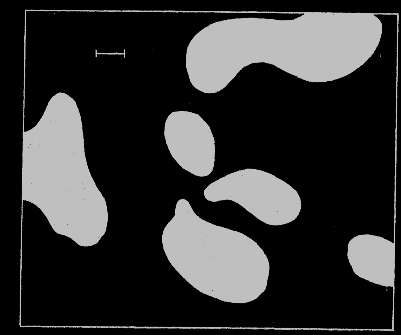
∂c=Δc+c(a−b) A picture from Turing's original paper
A picture from Turing's original paper
Dappling pattern emergence
Dappling pattern emergence
Reaction-Diffusion PDE
Reaction-Diffusion PDE
Diffusion PDE
Diffusion PDE
To play with this: see the website of Karl Sims
To play with this: see the website of Karl Sims
(or you can use PyCA!)
(or you can use PyCA!)
Some Solitons with Reaction-Diffusion Models
Some Solitons with Reaction-Diffusion Models
Some progress towards gliders?
Some progress towards gliders?
Belousov-Zhabotinsky with r,g,b
Belousov-Zhabotinsky with r,g,b
Belousov-Zhabotinsky in the physical world (experiment by Tim Kench)
Belousov-Zhabotinsky in the physical world (experiment by Tim Kench)
Various phases of the Gray-Scott Equation
Various phases of the Gray-Scott Equation
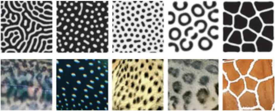
Some Patterns in Nature
Some Patterns in Nature
Some pattern simulations vs animal skin
Some pattern simulations vs animal skin
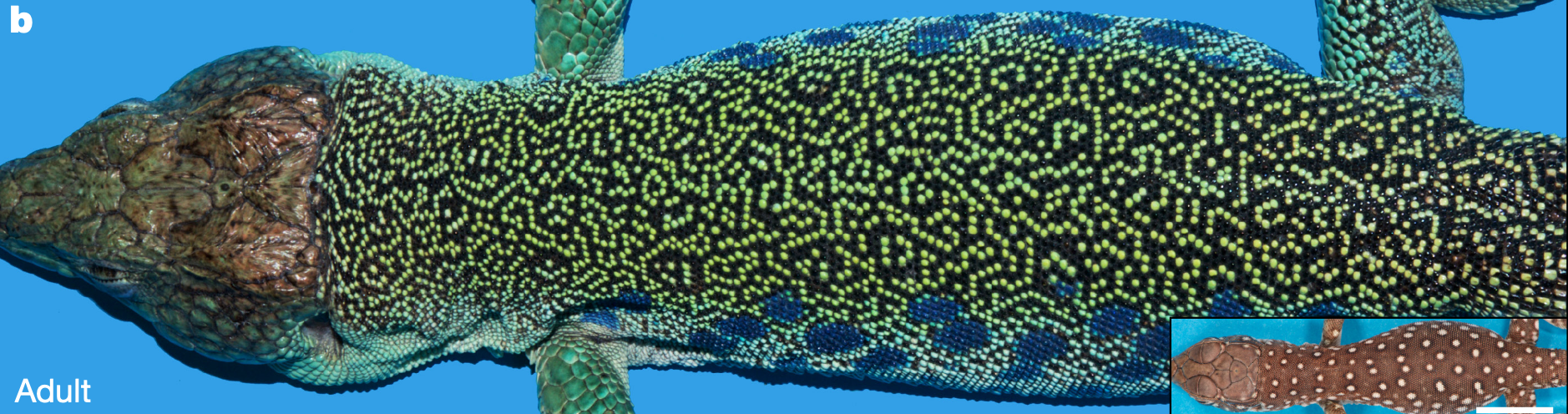
Some patterns on lizards scales (Manyukan, Montandon, Fofonjka, Smirnov, Milinkovitch from Unige)
Some patterns on lizards scales (Manyukan, Montandon, Fofonjka, Smirnov, Milinkovitch from Unige)
Key Statement (Informally)
Key Statement (Informally)
We don't need more than basic chemistry to explain the process of pattern formation
We don't need more than basic chemistry to explain the process of pattern formation
Diffusion: running the discrete Laplace's equation
Diffusion: running the discrete Laplace's equation
.